🐍 Stop trusting the Sharpe ratio

Replace total volatility with downside deviation using NumPy

Each week, I send out one Python tutorial to help you get started with algorithmic trading, market data analysis, and quant finance. Upgrade to a paid plan to access the code notebooks.

---

In today’s post, you’ll learn to compute the Sortino ratio in Python and compare assets through time.

What the Sortino ratio measures

The Sortino ratio measures risk-adjusted return using only the volatility of negative returns as the risk term.

It grew out of work by Frank Sortino in the 1980s and 1990s, as investors pushed back on treating upside and downside volatility as equally “bad.” It stuck because real traders often care more about losses and drawdowns than about choppy upside moves.

How pros use it

On a quant desk, the Sortino ratio is one of the quickest ways to sanity-check whether a strategy’s returns are “paid for” with too many bad days. It shows up in research next to Sharpe, max drawdown, and rolling performance charts, because no single metric tells the full story.

Risk teams also like downside-focused measures when they review products that can look stable most days and then gap down in stress.

If you’ve ever looked at equity curves that climb steadily and then give back months of gains in a week, you’ve seen why focusing on negative-return dispersion can be more informative than total volatility.

In practice, you’ll compute daily returns, subtract an optional benchmark return if you want an excess-return version, and then annualize both the mean return and the downside deviation.

In Python, the trick is to clip returns at zero so you keep only the negative part, square it, average it, and take the square root to get downside deviation.

Why it matters for beginners

Once you can compute a Sortino ratio, you can compare two assets that have similar Sharpe ratios and still see which one punishes you more on down days. You also get a reliable way to evaluate strategy tweaks without accidentally rewarding a version that simply has more upside noise.

The real payoff is that you’ll start diagnosing performance with data rather than vibes, especially when rolling windows show the metric drifting across regimes.

Let’s see how it works with Python.

Library installation

Install the libraries we need to download market data and compute downside-risk metrics in the same environment as the notebook.

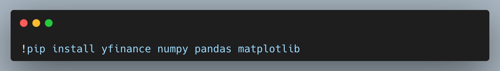
We use pandas and matplotlib even though they are not explicitly imported, because yfinance returns pandas objects and the .plot() call relies on matplotlib behind the scenes.

Imports and setup

Import numpy for fast math and yfinance to fetch historical prices for tickers like “SPY” and “AAPL” directly into pandas DataFrames.

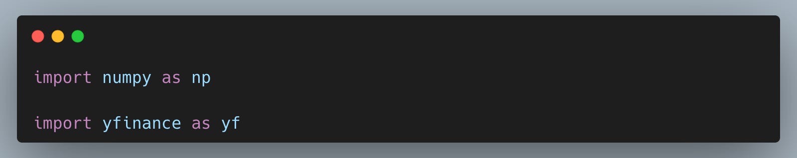
Keeping imports minimal makes it easier to see what the workflow depends on, which helps when you later move this from a notebook into a research script or a backtest engine.

Download prices and compute returns

Pull market data for “SPY” and “AAPL” over a fixed window so we can compare strategies/assets using the same dates and sampling frequency.

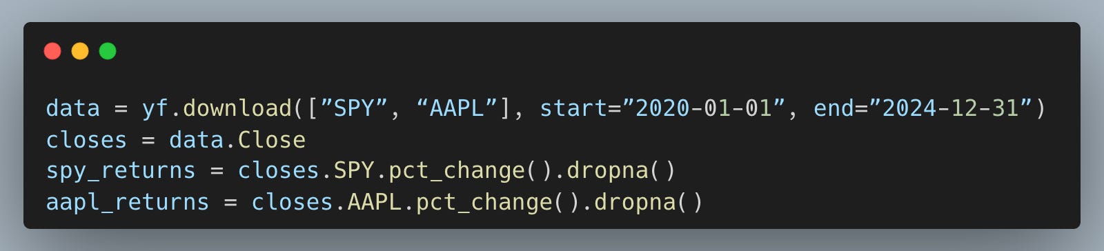
Working with daily percentage returns is the standard input format for ratios like Sharpe and Sortino, because it lets us summarize distribution shape rather than price level. Dropping the first NaN avoids propagating missing values into our risk metric.

Define the Sortino ratio function

Package the Sortino calculation into a reusable function so we can apply it to multiple assets and later to rolling windows without rewriting the logic.

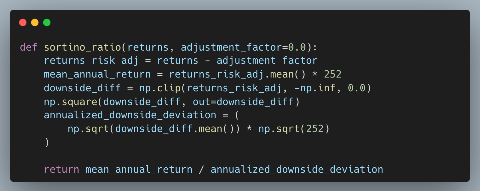
This implementation matches the post’s core idea: we treat upside volatility as neutral and measure “risk” using only negative-return dispersion. The adjustment_factor lets us turn this into an excess-return Sortino (for example, subtracting a constant daily cash rate), which is closer to how you’d compare strategies against a hurdle or benchmark in practice.

Compare levels and rolling behavior

Visualize how AAPL’s downside-adjusted performance changes over time relative to SPY.

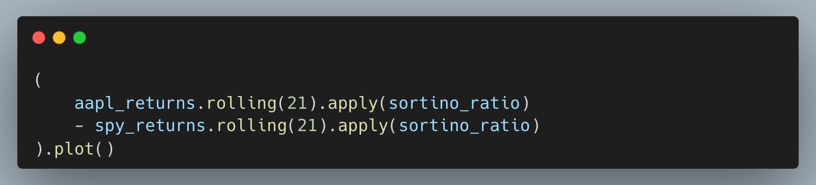
A single ratio over the full sample can hide regime shifts, which is exactly how two assets can look “similar on Sharpe” while feeling very different during drawdowns.

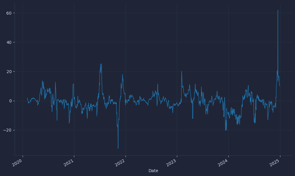
The result is a chart that looks like this.

Rolling Sortino makes downside-risk visible through time, and the difference helps us reason about consistency: we’re not just asking “who wins on average,” but “how often does one have better bad-day behavior than the other.”

Your next steps

You can now compute the Sortino ratio in Python and track it on a rolling basis to compare assets or strategy variants through time. That gives you a downside-focused check when Sharpe looks similar, so you can pick the version that avoids getting paid with too many bad days.