How to compute daily VaR fast

Skip big models, use covariance and weights

Subscribers, look for the code in your Private chat. Looking for the code notebooks? Consider a free subscription.

Value at Risk estimates the worst expected loss over a time horizon at a chosen confidence level.

Banks adopted VaR in the 1990s after JP Morgan released RiskMetrics with a variance-covariance framework for market risk.

Regulators and trading desks kept it because it is explainable, fast to compute, and broadly comparable across books.

How pros use it

Today, teams use VaR to size positions and set limits that match their mandates daily.

A quant desk pulls returns, estimates a covariance matrix, then computes portfolio volatility from weights under a normal assumption. They convert volatility into VaR at multiple horizons using square root of time, and monitor breaches against limits and alerts. Backtesting compares predicted losses to realized outcomes, flags underestimation during stress, and triggers model or limit adjustments after repeated misses.

Why you should care

For beginners, VaR turns vague risk ideas into concrete loss numbers you can act on.

You will size positions with a target loss in dollars, so stop guessing and start testing against history. You will catch data issues early because VaR jumps when returns spike or weights misalign during rebalances.

Let’s see how it works with Python.

Library installation

Install the packages needed to fetch data, compute statistics, and visualize results so the notebook runs end to end anywhere.

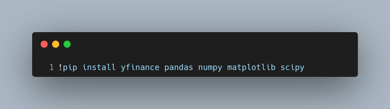
Installs inside notebooks can take a minute and version differences can change numerical results slightly, so pin versions for reproducibility in production. If you run this outside notebooks, install these packages once in your environment rather than in-line.

Imports and setup

We use pandas for tabular time series handling, numpy for vectorized math, scipy.stats.norm for normal quantiles, matplotlib.pyplot for plotting, and yfinance to download historical prices.

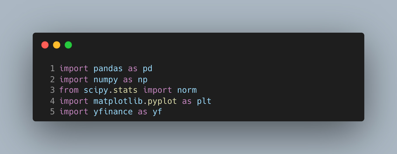
These imports cover a classic variance–covariance VaR workflow: retrieve prices, compute returns and covariances, then map volatility into loss bounds. Keeping this set minimal helps you focus on the model assumptions rather than tooling.

Define portfolio and pull prices

Specify a simple equity portfolio, set a dollar size, choose a one-sided tail probability, and fetch historical closing prices to anchor risk in real market data.

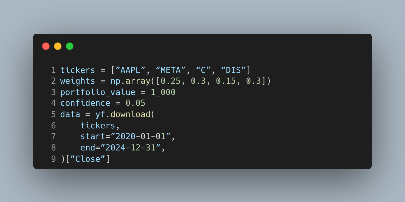
This step ties VaR to positions you could actually hold, which keeps the later loss number actionable in dollars. We use a 5% left-tail probability, which corresponds to a 95% one-day VaR under a one-sided view. For production, prefer adjusted prices (“Adj Close”) to handle splits/dividends cleanly and avoid distorted returns.

Estimate risk and compute VaR

Convert prices to returns, estimate the portfolio’s mean and covariance, then compute one-day variance–covariance VaR under a normal assumption.

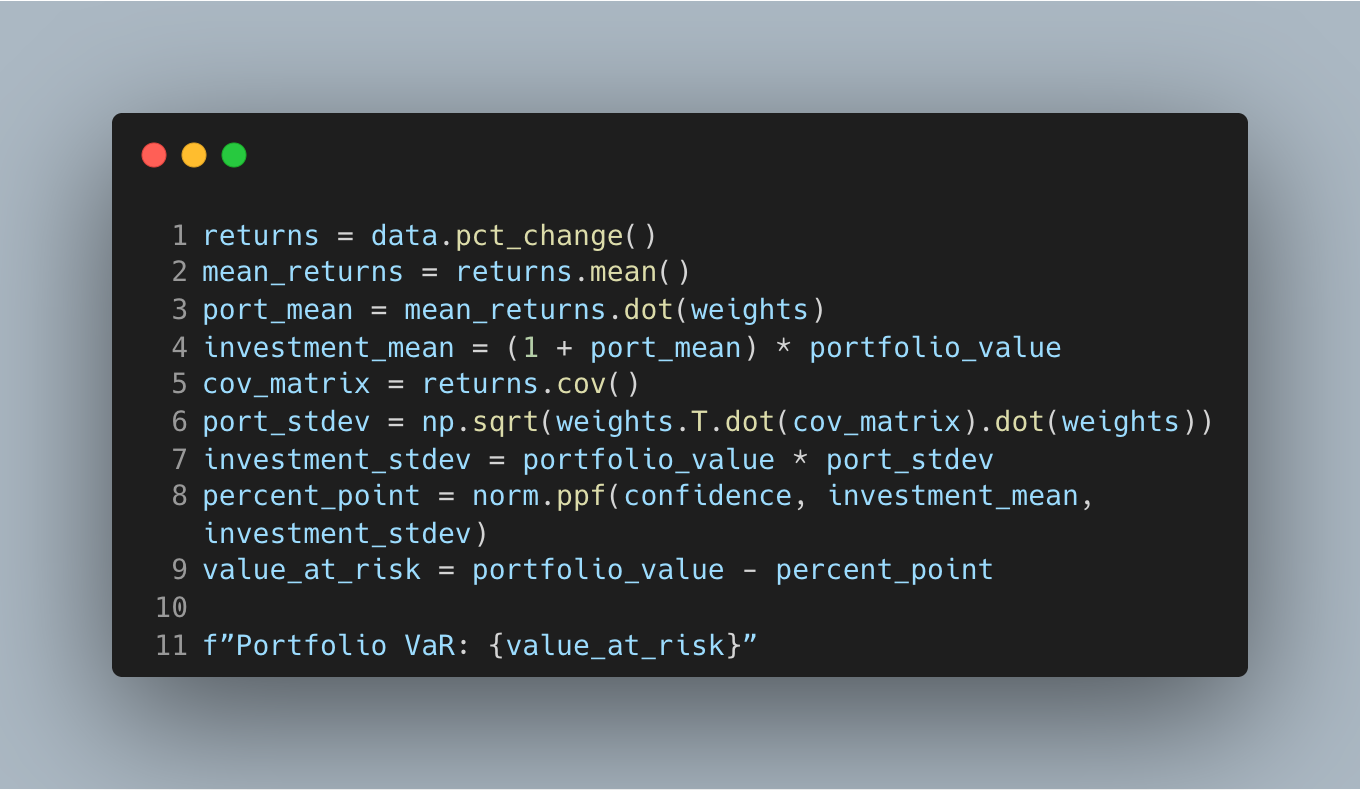
This is the desk-standard VaR pipeline: covariance aggregates co-movement across names and weights map that risk into your dollars. The normal model is fast and explainable; at daily horizons, the mean is small and volatility drives the tail. Treat this as a baseline you can backtest against realized losses to spot underestimation during stress.

Scale horizon and visualize losses

Extend the one-day VaR to multiple days using square-root-of-time scaling to get quick, comparable limits across horizons.

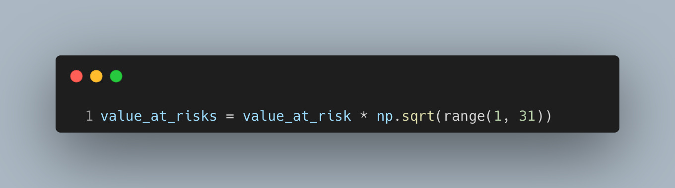
The sqrt(T) rule assumes independent, identically distributed returns with stable volatility, which is a decent first pass but can break in clustered volatility or trending markets. Use it for daily limit-setting and monitor exceptions; if breaches repeat, tighten limits or upgrade the model.

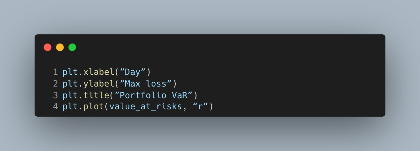
Plot the multi-day VaR curve so we can see how the expected worst loss accumulates as holding period increases.

The result looks something like this:

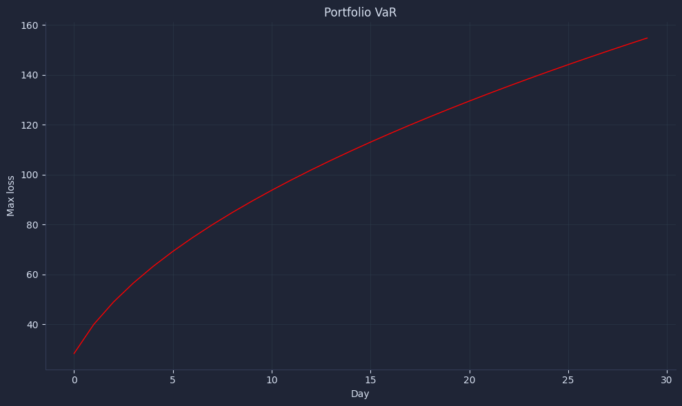
A simple plot communicates risk: how many days until losses reach your tolerance at the chosen confidence.

This makes risk sizing tangible and encourages limit discussions before a selloff, not during one. In practice, pair this with alerts and exception tracking to close the loop between prediction and realized outcomes.

Your next steps

Now you can compute one-day and multi-day VaR in Python from clean returns and weights, translate it into dollar loss, and tie it to position size and limits. Use it to backtest, monitor breaches, and adjust exposure so routine gaps stay within tolerance and decisions stay disciplined.