
🐍 Compute Sharpe the right way
Compute Sharpe from excess returns and sample volatility using pandas
Each week, I send out one Python tutorial to help you get started with algorithmic trading, market data analysis, and quant finance. Upgrade to a paid plan to access the code notebooks.

Sharpe ratio basics
The Sharpe ratio measures excess return per unit of volatility, letting you compare strategies on a risk adjusted basis.
William Sharpe introduced it in the 1960s to evaluate portfolios relative to a risk free benchmark return stream. It spread through modern portfolio theory and became a standard yardstick for funds, allocators, and regulators over decades.
How pros use it
Professionals use Sharpe daily to rank strategies and budget risk, then monitor stability through time windows.
They compute daily excess returns versus cash and annualize by square root of 252, then track rolling windows for drift. Desks compare Sharpe at equal leverage by de-risking exposures and subtracting financing costs, then align calendars across assets and markets. They set guardrails when rolling Sharpe falls and investigate drawdowns, then test whether improvements survive costs and slippage assumptions.
A few details matter if you want clean numbers that hold up under review. Use excess returns that subtract a realistic cash rate for the period you measure, not a fixed zero if rates moved. Match sampling across series so you do not compare daily to weekly noise, and use close-to-close returns if your holdings are end-of-day. Prefer sample standard deviation on noncumulative returns, watch for missing data that creates artificial spikes, and annualize using an appropriate trading-day count for your market.
Why beginners care
Learning Sharpe early gives you a clean way to compare ideas without guessing or hype.
You will reduce false positives and spot fragile strategies, then focus on hypotheses that deliver steadier efficiency over time. You will also practice good habits like using excess returns and choosing sensible windows, then avoid lookahead mistakes in backtests.
Let’s see how it works with Python.
Library installation
Install the libraries we need to fetch market data, compute statistics, and visualize results so this notebook runs cleanly anywhere.
Imports and setup
We use yfinance to pull historical prices, numpy for fast numerical operations such as annualization, and matplotlib.pyplot to visualize Sharpe behavior over time.
Keeping imports minimal helps us focus on the Sharpe workflow without extra dependencies. This mirrors what pros do in quick analyses: load prices, compute stats, and plot diagnostics. It also makes results easier to reproduce across machines and environments.
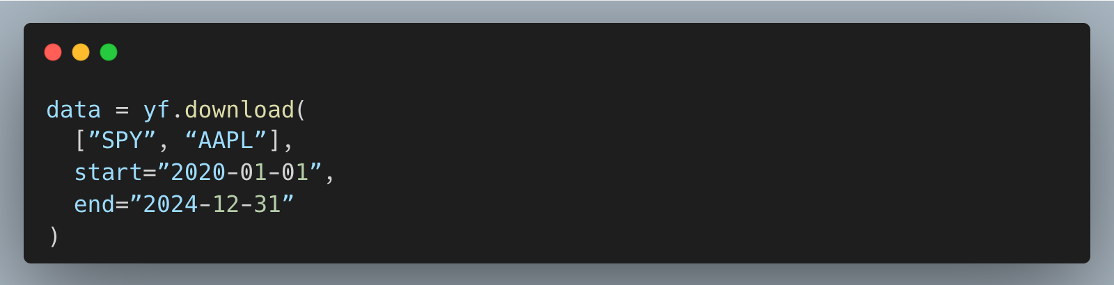
Download and prepare daily returns
Pull adjusted close prices for SPY and AAPL over a fixed horizon so we compare assets on the same calendar and sampling frequency.
Using a single source avoids mismatched calendars and survivorship issues that skew risk metrics. Adjusted prices account for splits and dividends, which is important when you want returns that reflect what holders experienced. Consistent sourcing reduces noisy differences that would otherwise leak into Sharpe comparisons.
Convert prices to noncumulative daily returns using close-to-close changes, which is the correct input for Sharpe.
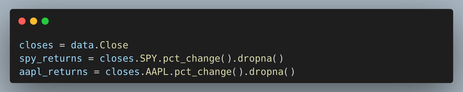
We compute simple daily returns because Sharpe expects a stream of noncumulative observations; the difference versus log returns is negligible at daily horizons. Dropping missing values prevents artificial spikes or divide-by-zero artifacts that can inflate volatility. This gives us a clean, aligned return series for each asset.
Define and compute Sharpe ratios
Define a helper that computes an annualized Sharpe ratio from daily returns, with an optional constant daily cash adjustment for excess returns.
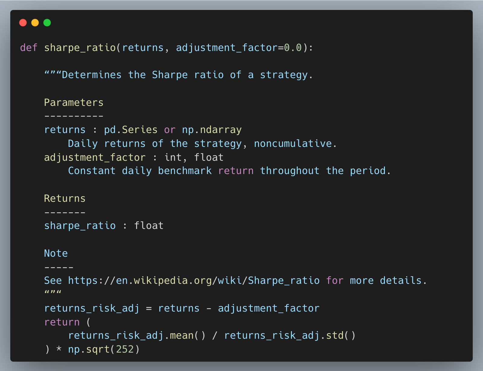
This implementation uses the sample standard deviation (pandas’ default) on noncumulative returns and annualizes with sqrt(252), matching common practice on U.S. trading days. In production, we would subtract a time-varying daily cash rate rather than a constant when rates move. The function enforces the “excess return per unit of volatility” idea that lets us compare assets fairly.
Compute full-sample Sharpe ratios for SPY and AAPL to benchmark their risk-adjusted performance over the same window.
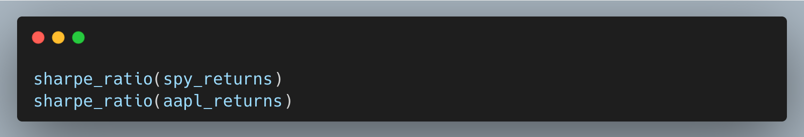
Looking at full-sample Sharpe gives a quick first pass on which asset delivered more return per unit of risk, unlevered and on identical sampling. This avoids the “bigger CAGR wins” trap by normalizing for volatility and frequency. Treat these as starting points before you inspect stability through time.
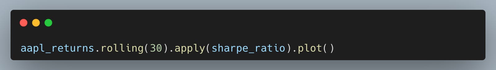
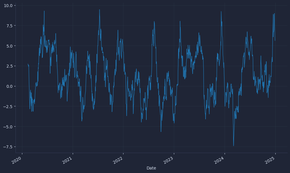
Visualize rolling Sharpe and differences
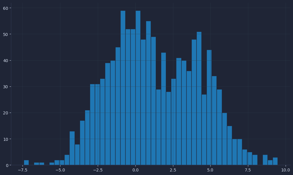
Track 30-day rolling Sharpe for AAPL, then plot its distribution and the rolling Sharpe difference versus SPY to see stability and relative edge.
The result is a chart that looks like this.
Now create a histogram to visualize the frequency.
The result is a chart that looks like this.
Finally, compare the two returns.
The result is a chart that looks like this.
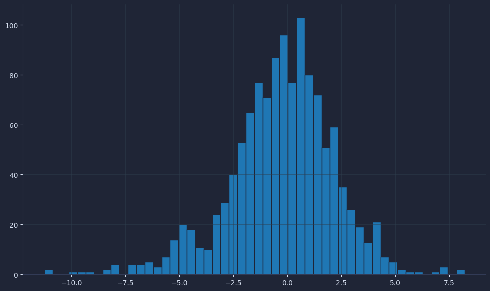
Rolling windows reveal regime shifts that a single full-period number hides, which is how desks set guardrails and monitor drift. The histograms show how often AAPL’s efficiency clusters at certain levels and when it outperforms SPY on a risk-adjusted basis. Short windows can be noisy, so in real reviews we also test multiple horizons and subtract a realistic daily cash rate when conditions change.
Your next steps
You can now compute Sharpe from excess returns, annualize correctly, and read rolling windows to compare strategies on equal risk. Use it to cut noisy ideas quickly, budget leverage with a clean yardstick, and track stability across regimes so your allocations favor strategies that hold up after costs.