🐍 A simple risk model helps

Build risk parity weights with Riskfolio-Lib and yfinance data

Each week, I send out one Python tutorial to help you get started with algorithmic trading, market data analysis, and quant finance. Upgrade to a paid plan to access the code notebooks.

---

In today’s post, you’ll build a risk parity portfolio in Python and then add a return constraint.

What risk parity means

Risk parity is a portfolio construction method that sets position sizes so each asset contributes a similar share of total portfolio risk.

It became widely known after Bridgewater scaled the idea in the 1990s and showed it could run in large, diversified portfolios. Since then, the concept has spread because it translates a common-sense goal into something you can measure and optimize.

How pros use it

Modern systematic teams use risk parity as a sizing layer that sits underneath their signals and forecasts.

In practice, the workflow starts with clean daily returns, then a covariance estimate that is consistent with your trading horizon. From there you solve for weights that equalize risk contributions, which prevents one volatile name from dominating PnL even if you “diversify” by ticker count. Libraries like Riskfolio-Lib make this approachable, but the professional habit is the important part, you always validate the result by checking risk contributions, not just looking at weights.

Why it helps beginners

Once you can build a risk parity portfolio, you stop confusing “number of holdings” with diversification, and your backtests get easier to interpret.

You also get a practical framework for handling the problem you will hit immediately in real data, different stocks have different volatilities and correlations, so naïve weights create accidental concentration. When you add a minimum return constraint, you also see the real tradeoff, forcing more expected return usually breaks perfect risk equality, and you can quantify that instead of guessing.

Let’s see how it works with Python.

Library installation

Install the third-party libraries used in this notebook so you can download market data and run the risk parity optimizer locally.

Riskfolio-Lib depends on scientific Python packages (like NumPy, pandas, SciPy, and CVXPy) that pip will usually pull in automatically, but some environments need compilers or platform-specific wheels. If installation fails, try a fresh conda environment or follow the Riskfolio-Lib docs for your OS.

Imports and setup

We use warnings to silence noisy library output, yfinance to fetch historical prices from Yahoo Finance, and riskfolio (Riskfolio-Lib) to estimate covariances and solve the risk parity optimization.

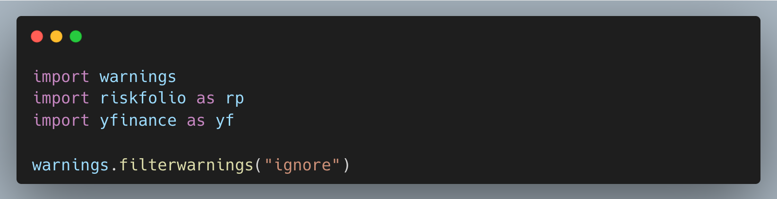
Filtering warnings keeps the notebook output readable while we iterate on portfolio sizing ideas, but it can also hide useful diagnostics during troubleshooting. If you run into unexpected results, consider removing this line so you can see numerical and data warnings.

Build a clean returns matrix

Define the investable universe, fetch adjusted close data with yfinance, and convert prices into daily returns that the risk model can work with.

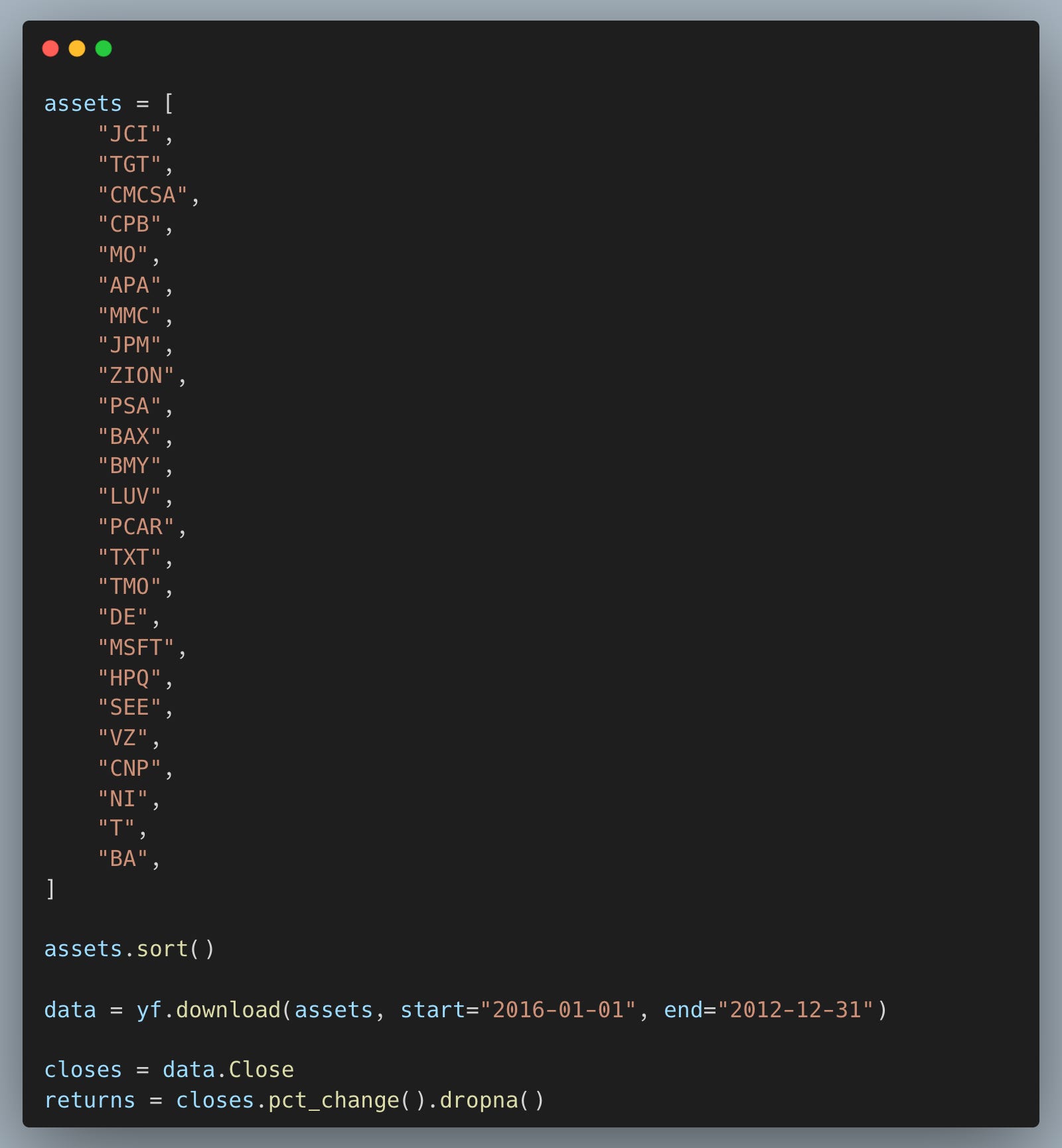
Risk parity is only as good as the returns matrix we feed it, so getting aligned daily returns is the real “data engineering” step here. Using pct_change() gives simple (non-log) returns, which is a common choice for covariance-based risk models at daily frequency.

Estimate risk model inputs

Create a Riskfolio-Lib Portfolio object and estimate expected returns and the covariance matrix from historical data.

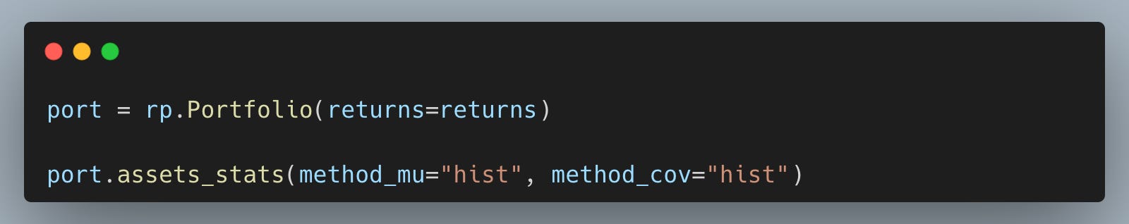
This is where we separate “signals” from “sizing”: even with no alpha model, we still need a defensible covariance estimate to understand concentration. Using method_cov=”hist” keeps the example simple, but in real workflows you’d compare alternatives (EWMA, shrinkage) because covariance estimation drives risk contributions.

Solve risk parity weights

Optimize for risk parity weights using historical scenarios, then re-run with a minimum return constraint to show the tradeoff between return targeting and equal risk contribution.

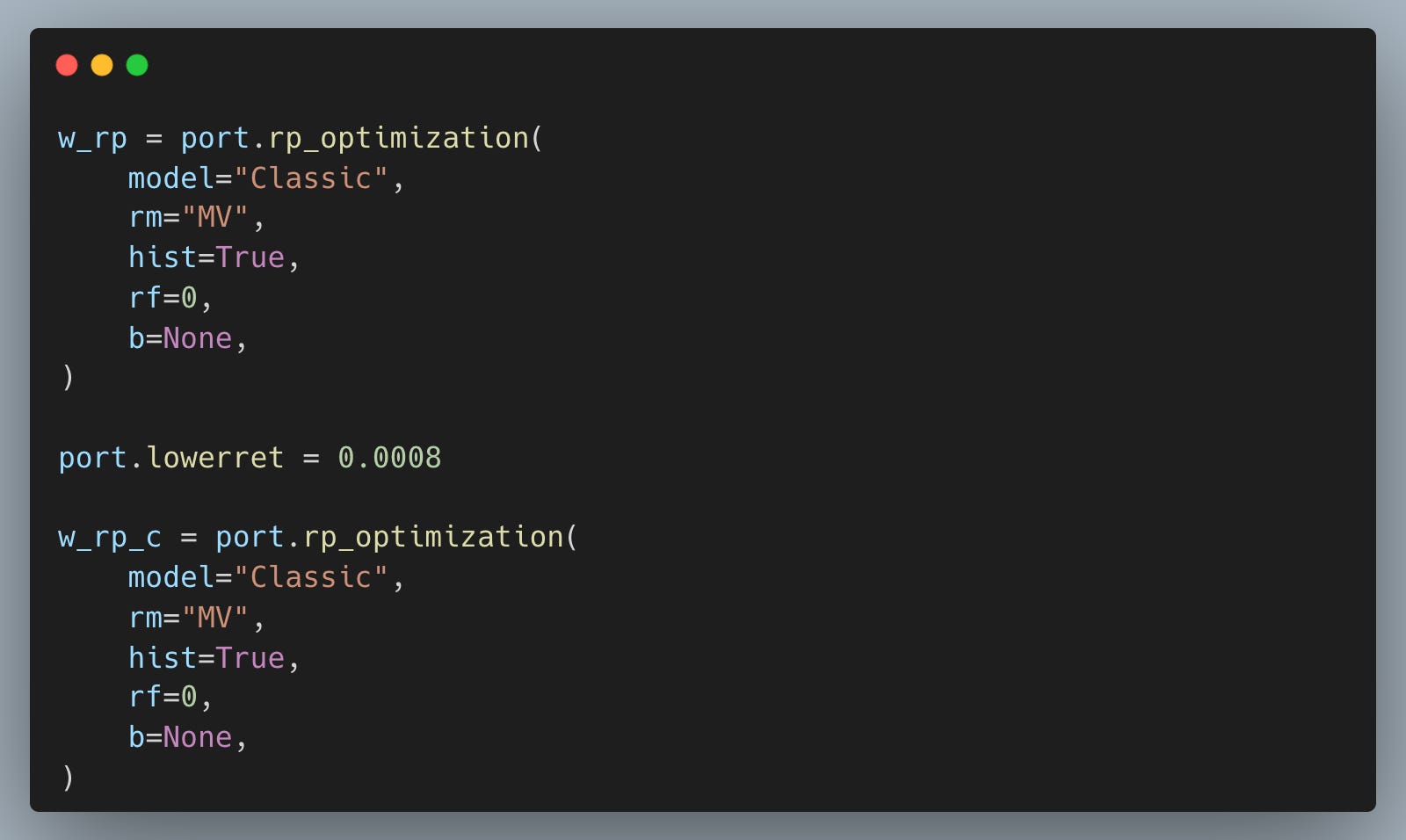
The unconstrained solution is the “pure sizing layer” that tries to keep one volatile stock from silently dominating portfolio swings. Adding port.lowerret forces the optimizer to chase a minimum expected return, which typically breaks perfect equality in risk contributions, and that’s exactly the point: we can measure the compromise instead of guessing.

Visualize weights and risk contributions

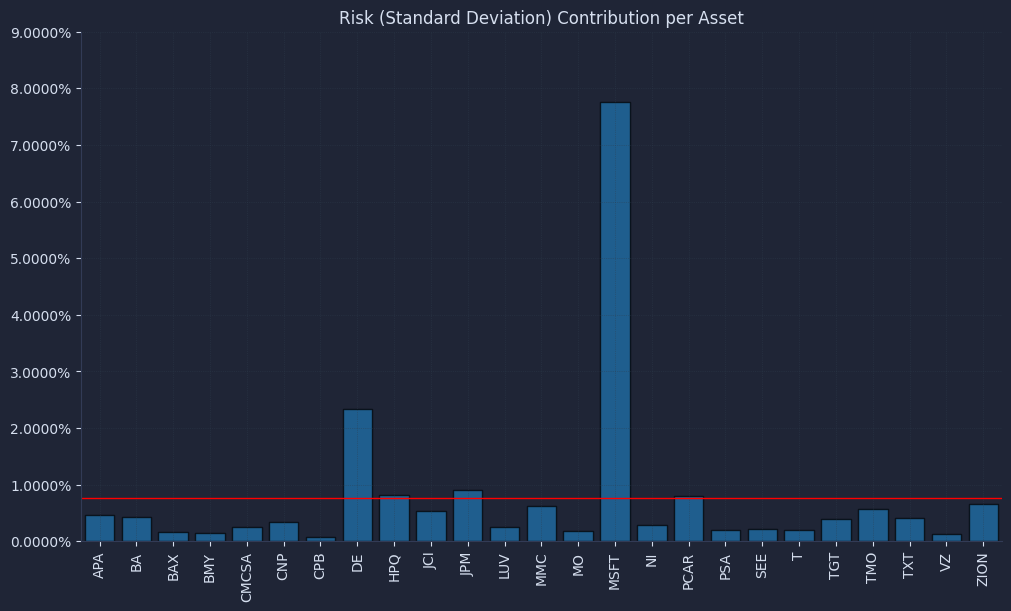
Plot weights and risk contributions for both portfolios so we validate diversification in risk terms rather than trusting the weight vector.

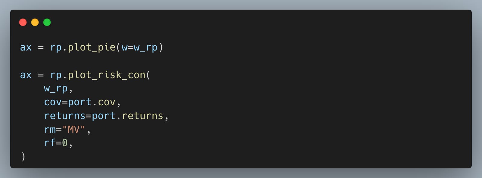
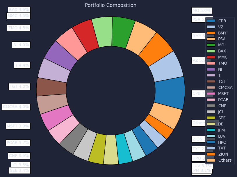
The result is a chart that looks like this.

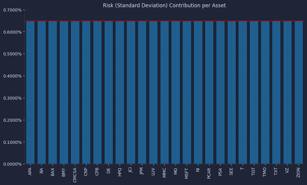
Then we can check how the risk contribution changes when adding a lower return constraint.

The result is a chart that looks like this.

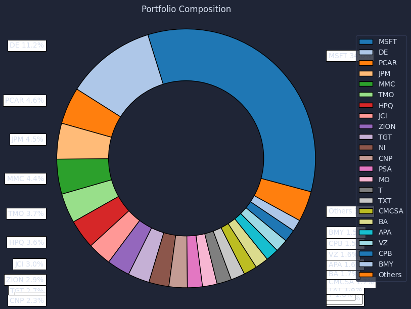
The pie charts can look “diversified” in both cases, but the risk contribution plot is the professional check that answers the real question: who is driving our PnL variance. This validation step is what helps us stop confusing “many tickers” with “many independent bets,” especially once constraints start pushing the optimizer away from equal risk.

Your next steps

You can now build a risk parity portfolio in Python, validate it by checking risk contributions, and then add a minimum return constraint to see how sizing changes. This matters because it keeps one or two volatile names from dominating PnL and makes your backtests reflect the signal, not accidental concentration.